In the steps below, 🖱 means a left mouse click (🖱🖱 a double click) and → leads to the next action. Labels in the screenshots are those of the ANSYS Workbench interface.
1. Analysis model and input data
Analysis model
Loading diagram in the XYZ coordinate system of the ATD
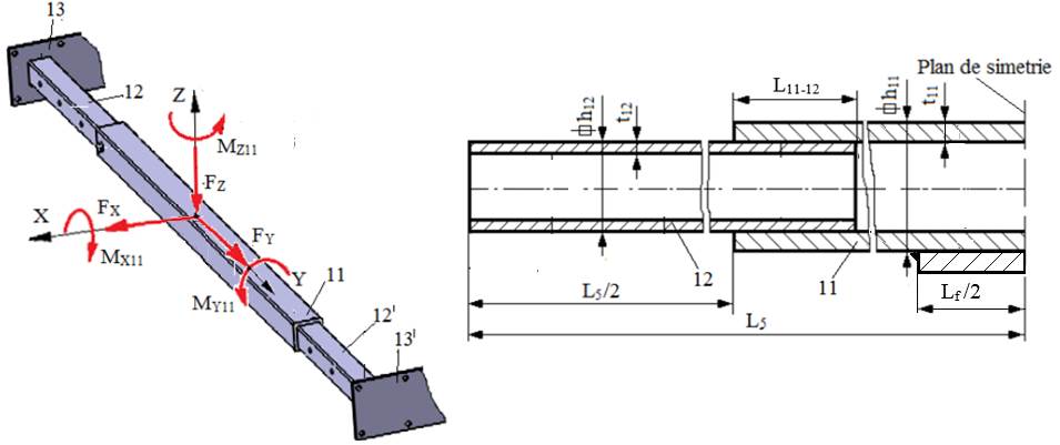
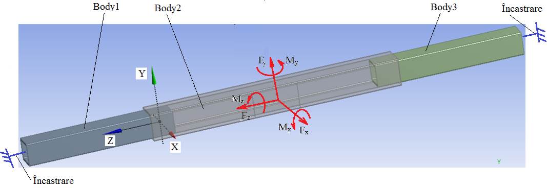
Geometric model in the ANSYS coordinate system
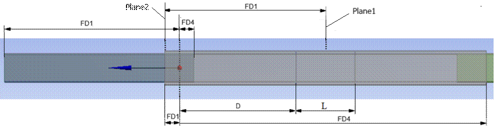
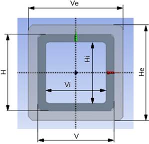
Geometric parameters in ANSYS
Input data (Ex.6.1, Ex.6.2)
Forces: FX = 1500 N, FY = 300 N, FZ = 700 N.
Moments: MX11 = 75000 Nmm, MY11 = 585000 Nmm, MZ11 = 90000 Nmm.
Geometric parameters: L11 = 550 mm; L11-12 = 70 mm; h12 = 50 mm, t12 = 5 mm, h11 = 60 mm, t11 = 5 mm; Lf = 120 mm.
Material: S235, weldable general-purpose steel.
Operating constraints: temperature T = (−30…40) °C.
Parameters of the ANSYS model
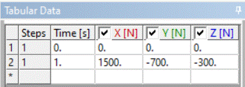
Forces: Fx = FX = 1500 N, Fy = −FZ = −700 N, Fz = −FY = −300 N.
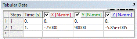
Moments: Mx = −MX11 = −75000 Nmm, My = MZ11 = 90000 Nmm; Mz = −MY11 = −585000 Nmm.
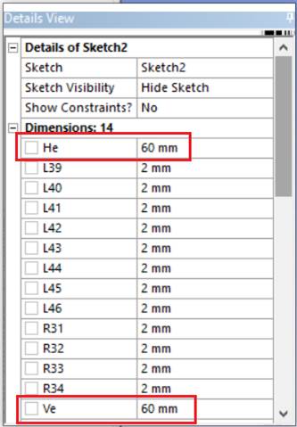
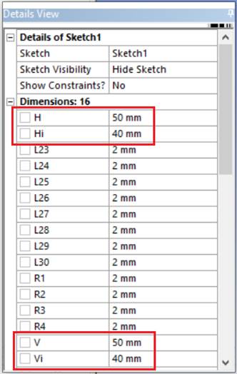
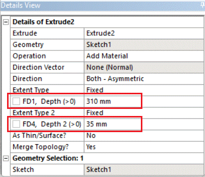
Geometric parameters: He = 60 mm, Ve = 60 mm, H = 50 mm, V = 50 mm, Hi = 40 mm, Vi = 40 mm; for Body1 (Body3): FD1 = 310 mm and FD4 = 35 mm; for Body2: FD1 = 35 mm and FD4 = 515 mm; for Plane1: FD1 = 240 mm; for the support footprint (relative to Plane2): D = 215 mm and L = 120 mm.
Material: S235, weldable general-purpose steel, with σat = σ02/c = 235/1.3 = 180 MPa (since the FEA model is more accurate, a lower safety factor c = 1.3 was adopted than for the classical, less accurate design models); allowable contact stresses: σas = 90 MPa, the allowable steel-on-steel normal crushing stress, and τas = 45 MPa, the allowable steel-on-steel tangential contact stress.
2. Entering the data in ANSYS (Annex.AN.1)
2.1 Launching the application
Downloading, saving and opening the application
FEA_11-12 → [unzip FEA 12-11.zip and save it].
Opening the Workbench (ANSYS) environment
🖱  → [the window
  opens].
Opening the project (application)
🖱 (
( ) → [select the folder FEA 12-11 containing the file (application)], [select the file name 🖱
 ]; the window
  of the previously developed project A opens, with its component modules:
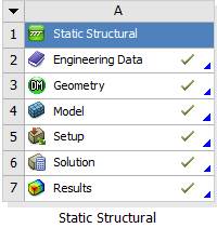
Note. All modules are up to date ( ).
).
2.2 Pre-processing
2.2.1 Changing the geometric parameters
Loading the DesignModeler module
🖱🖱 → the window
  opens with the geometric model.
Changing the dimensions
Changing the section dimensions
🖱 → 🖱
→ 🖱 →
→  : [change the dimensions He, Ve (fig. a)].
🖱 → 🖱 → : [change the dimensions Hi, Vi, H, V (fig. b)].
a b
Changing the extrusion lengths
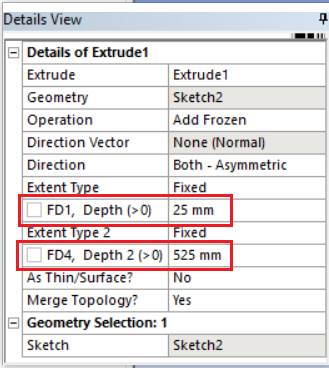
🖱 → : [change the dimensions FD1, FD4 (fig. a)].
🖱 → : [change the dimension FD1 (fig. b)].
a b
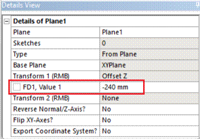
Changing the position of the symmetry plane
🖱 →
→  : [change the dimension FD1].
Changing the dimensions of the loading surface
🖱 → 🖱
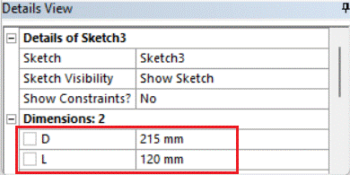
→ 🖱 → : [change the dimensions D, L].
Saving the project and returning to the main window
🖱 → 🖱
→ 🖱 (the window
  with project A appears).
2.2.2 Changing the parameters of the FEA model
Loading the Static Structural module
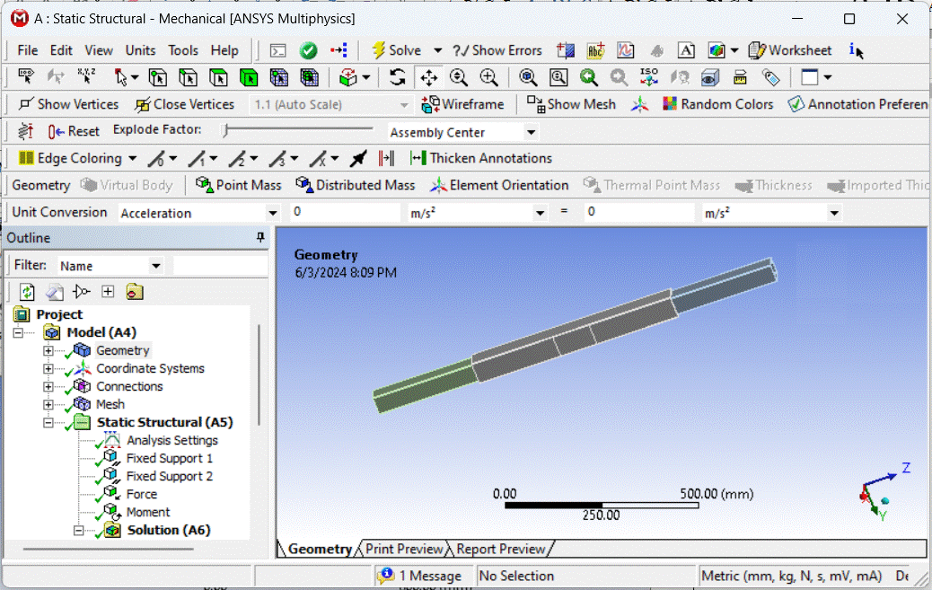
🖱🖱  → the window
  opens with the FEA model:
Updating the geometric model

 → 🖱
→ 🖱 (the modified geometric model appears).
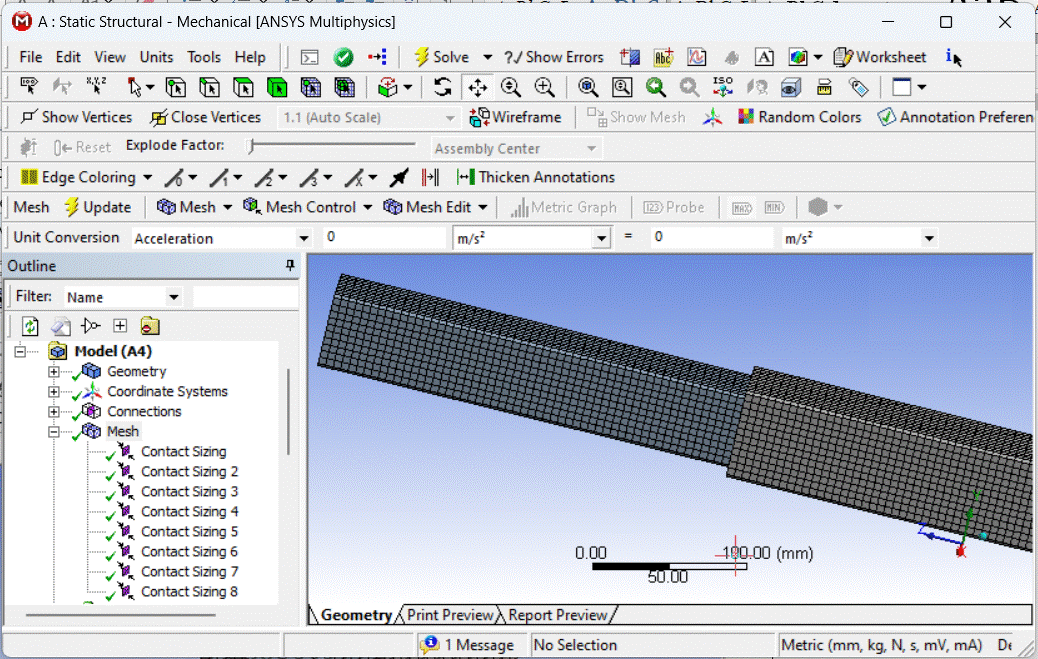
Meshing the model
 → 🖱
→ 🖱 ; the FEA model appears.
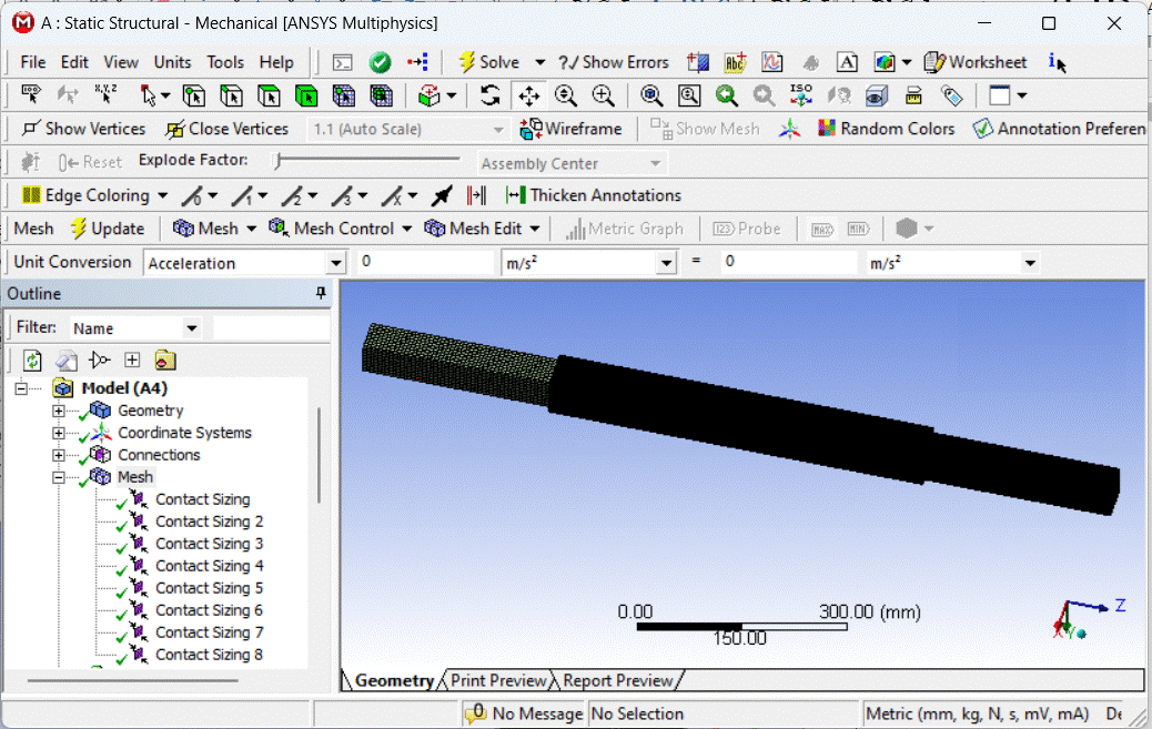
Note. This FEA model was generated with the default meshing parameters. These usually produce a large number of nodes and therefore a much longer solving time, especially on computers with limited hardware. To reduce the solving time, the meshing parameters can be changed and the model re-meshed, as in the next step.
Changing the meshing parameters and re-meshing (if needed)
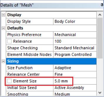
– changing the finite element size for the bodies,
🖱 → 🖱
→ 🖱 →
→  : 🖱
: 🖱 , [activate the option 🖱🖱
 and change the value in the right-hand column, e.g. 5.0 (fig. a)];
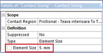
– changing the finite element size in the contact zones,
🖱 → 🖱 →
→  : [activate the option 🖱🖱 and change the value in the right-hand column, e.g. 5.0 (fig. b)] (repeat this sequence for the groups
  ,
,  ,
,  …
…  ).
).
a b
– re-meshing with the changed parameters,
→ 🖱 (the modified FEA model appears).
Changing the loads
🖱 .
.
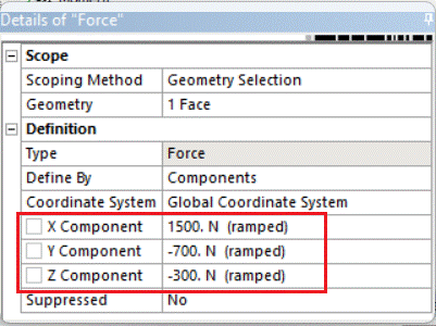
Changing the forces
🖱 →
→  : [change the values
  ,
,  ,
,  , e.g. 1500, −700, −300 (fig. a)].
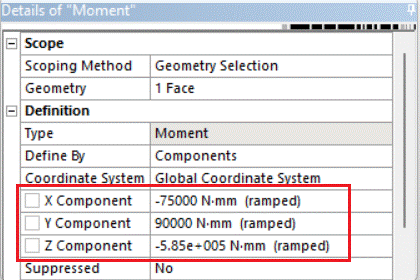
Changing the moments
🖱 →
→  : [change the values
  , , , e.g. −75000, 90000, −585000 (fig. b)].
a b
🖱 → 🖱
→ 🖱 .
.
3. Solving and saving the model
 → 🖱
→ 🖱 .
.
4. Results and checks
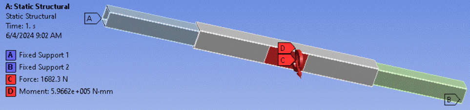
Viewing the loads and reactions
Viewing the applied forces and moments
🖱
🖱
🖱
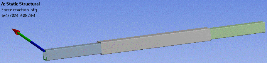
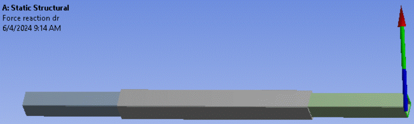
Viewing the forces in the reaction zone
🖱

🖱

🖱
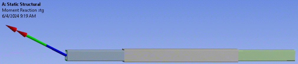

🖱
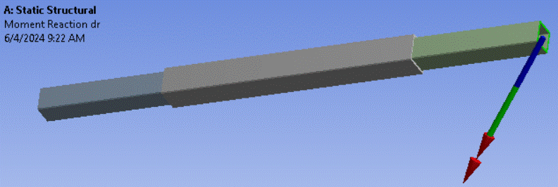

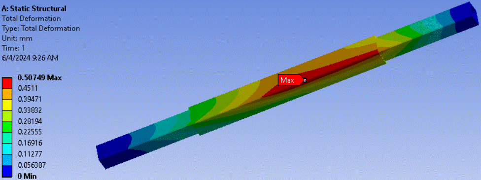
Viewing the displacements
🖱 → the model appears
Viewing the stresses
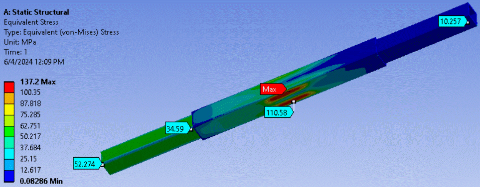
Equivalent stresses on the global model
🖱  → 🖱
→ 🖱 (marks local stress values at points) → [move the cursor and 🖱 click the point on the model where the stress value should be shown]; to delete a local value: 🖱
 (Label) → [🖱 select the value, then press the Delete key].
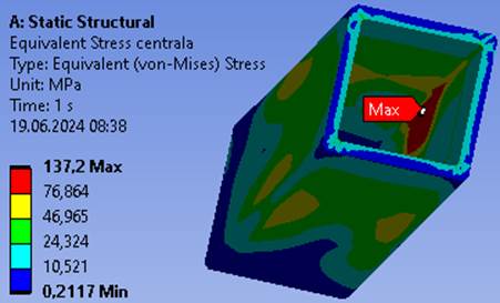
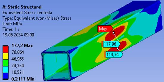
Equivalent stresses on the model of the central tube
🖱
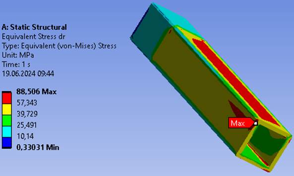
Equivalent stresses on the model of the right tube
🖱
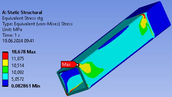
Equivalent stresses on the model of the left tube

Viewing the pressures and stresses in the contact zones
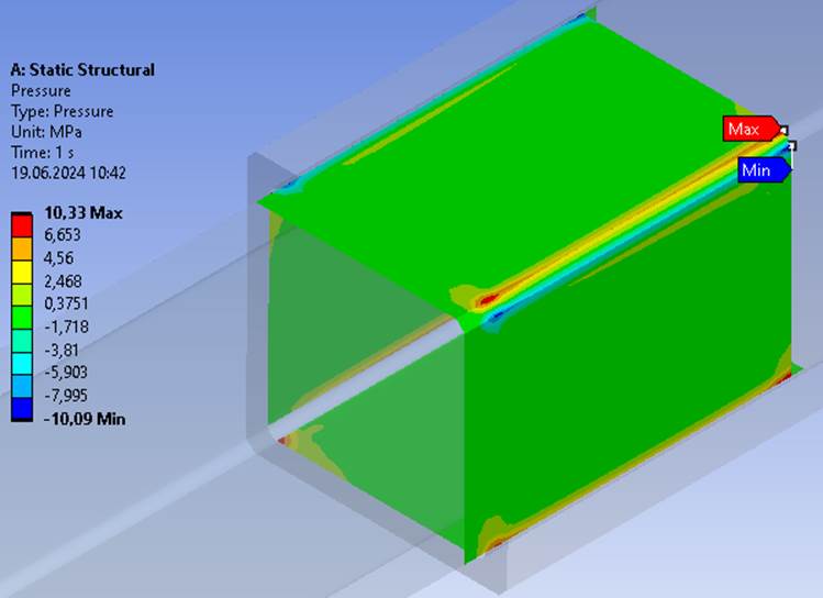
Pressures on the contact surfaces
🖱
🖱 ;
;
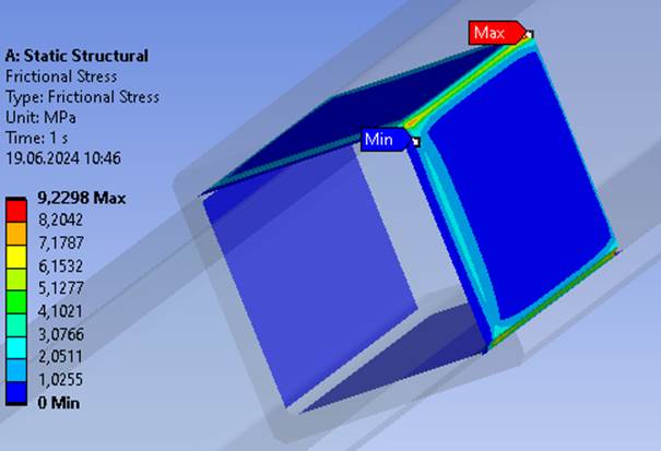
Tangential (friction) stresses on the contact surfaces
🖱 ;
;
Checks
Deformation check
δ ≤ δa; 0.507 ≤ 5 mm (satisfied).
Note. The allowable deflection is set by the operating conditions.
Equivalent (von Mises) stress check
σech_max ≤ σat; 137.2 > 132 MPa (NOT satisfied),
where σech_max is the maximum equivalent stress in the figure above.
If the inequality above is NOT satisfied, one of the following options can be chosen:
a. choose a better material;
b. change the cross-section geometry, taking larger values of the square side h11 and wall thickness t11 from Annex.ST.02, while keeping the inner dimension that contacts the inserted tube;
c. change both the material and the geometry.
Option a is adopted here: material S295 is chosen, so
σech_max ≤ σat; 137.2 < 295/1.3 = 226.9 MPa (satisfied).
Normal contact pressure check
pmax ≤ σas; 10.33 ≤ 90 MPa (satisfied),
where pmax is the maximum (absolute value) of the pressure in the figure above.
Tangential contact stress check
τmax ≤ τas; 9.23 ≤ 44 MPa (satisfied),
where τmax is the maximum tangential contact stress (frictional stress) in the figure above and τas the allowable tangential contact stress.